Database System Description¶

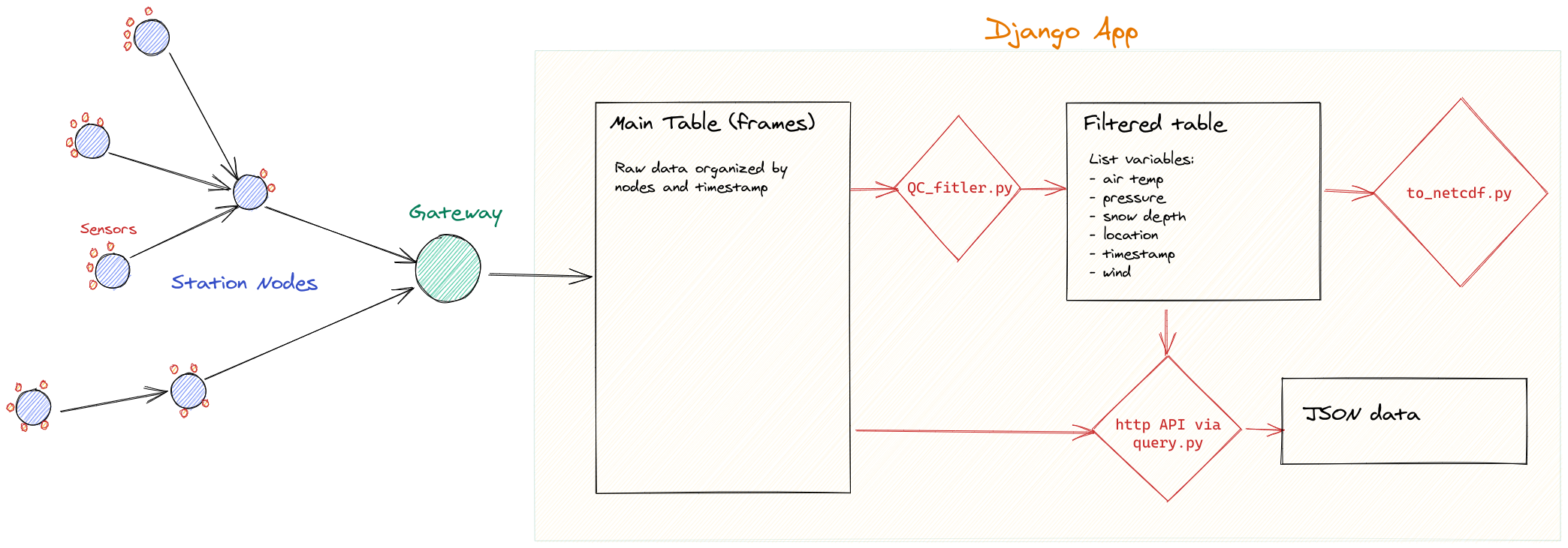
The General concept of the data pipeline consists of the sensors sampling at regular intervals predefined in each nodes. Data are stored locally and also put in a queue to be sent out via radio, 4G or Iridium. Data are then stored in a PostgreSQL database in raw format. This table is accessible by http queries using the API wsn_client (restricted access). Those data have no quality control and are stored as is. Currently under construction, data are then filtered, flagged for quality, and aggregated into a table. Those data are accessible in JSON format via http request (restricted access), or in the the case of the Svalbard network in netcdf4 format via the SIOS dataportal.

Download Data from SIOS Dataportal¶

[TBA]

Download Data Directly from the UiO Django App¶

Through Grafana¶

Data can be downloaded interactively via the Grafana interface. The Grafana portal requires login information.

go to the desired dashboard
define the time range
click on the panel title > more ... > export CSV
open your Download folder, here it is

Through `http` request¶

The Django database can be queried via http request, and return data organized in a json object. [write about the http request structure/fields]

Python query function¶

You will need a Python 3.7 environment with the libraries requests, and pandas installed.

Assuming you have Anaconda 3 installed on your machine, type the following in your terminal to create a suitable environment:

conda create --name uioData  python=3.8
conda activate uioData
conda install pandas requests ipython

# in case you use Jupyter Lab
conda install ipykernel
ipython kernel install --user --name=uioData

# other python package of interest for data processing
conda install numpy matplotlib scikit-learn

# cd to a good location to clone the WSN_CLIENT repository
git clone git@github.com:spectraphilic/wsn_client.git  #uses SSH key to query github otherwise use https: git clone https://github.com/spectraphilic/wsn_client.git

pip install -e [pathTo]/wsn_client     # point the pip install to where you cloned the wsn_client package

From there you will need to obtain a token from the database administrators, granting you access to the database via http. You need to add the TOKEN as an environment variable. On Unix system (Linux and MacOS) add to .bashrc file the line export WSN_TOKEN='xxxxx'. Replace the 'xxxxx' by the actual token. Then you should be able to access the TOKEN in a python console (after restarting you terminal) with the following Python command: TOKEN = os.getenv('WSN_TOKEN')

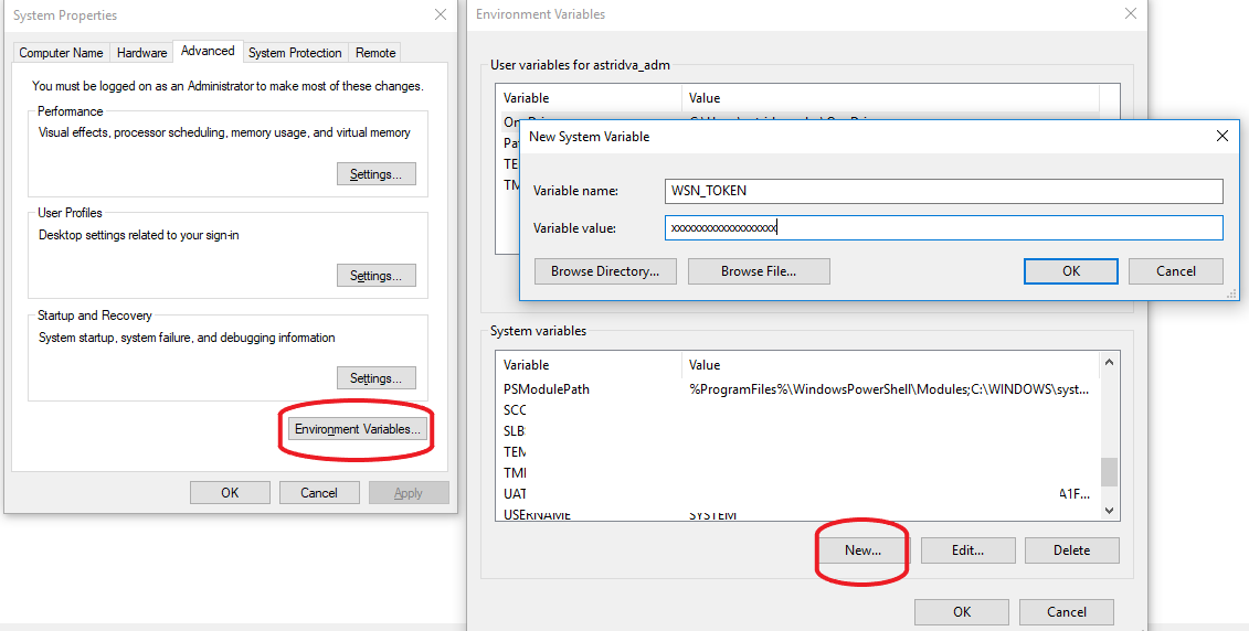
For Windows, you need to add the WSN_TOKEN to your environment variables. One way to do this is to right click PC -> Properties -> Advanced System settings -> Environment Variables

Windows screenshot

Brief example to download data¶

from wsn_client import query
import datetime, os

start = datetime.datetime(2019, 6, 1)
end = datetime.datetime(2019, 6, 15)

df_kong = query.query('postgresql', name='sw-002', time__gte=start, time__lte=end, limit=2000000000000)
df_kong.head()

Selecting data (rows)¶

First choose the database to pull data from, choices are clickhouse (for raw data from finse/mobile flux), and postgresql (for everything else). How data is selected depends on the database used. ClickHouse: query('clickhouse', table='finseflux_Biomet', ...). Choices for table are: finseflux_Biomet, finseflux_StationStatus, mobileflux_Biomet and mobileflux_StationStatus. PostgreSQL:

query('postgresql', name='eddypro_Finseflux', ...)
query('postgresql', serial=0x1F566F057C105487, ...)
query('postgresql', source_addr_long=0x0013A2004105D4B6, ...)

Data from PostgreSQL can be queried by any metadata information, most often the name is all you need.

Selecting fields (columns)¶

If the fields parameter is not given, all the fields will be returned. This is only recommended to explore the available columns, because it may be too slow and add a lot of work on the servers. So it is recommended to ask only for the fields you need, it will be much faster. Examples:

query('clickhouse', table='finseflux_Biomet', fields=['LWIN_6_14_1_1_1', 'LWOUT_6_15_1_1_1'], ...)
query('postgresql', name='eddypro_Finseflux', fields=['co2_flux'], ...)

The field ‘time’ is always included, do not specify it. It’s a Unix timestamp (seconds since the Unix epoch). The rows returned are ordered by this field.

Selecting a time range¶

Use the parameters time__gte and/or time__lte to define the time range of interest. The smaller the faster the query will run. These parameters expect a datetime object. If the timezone is not specified it will be interpreted as local time, but it’s probably better to explicitely use UTC. Example:

query(
    'clickhouse', table='finseflux_Biomet',
    fields=['LWIN_6_14_1_1_1', 'LWOUT_6_15_1_1_1'],
    time__gte=datetime.datetime(2018, 3, 1, tzinfo=datetime.timezone.utc),
    time__lte=datetime.datetime(2018, 4, 1, tzinfo=datetime.timezone.utc),
    ...
)

Limiting the number of rows¶

The limit parameter defines the maximum number of rows to return. If not given all selected rows will be returned. Example:

query(
    'clickhouse', table='finseflux_Biomet',
    fields=['LWIN_6_14_1_1_1', 'LWOUT_6_15_1_1_1'],
    time__gte=datetime.datetime(2018, 3, 1, tzinfo=datetime.timezone.utc),
    time__lte=datetime.datetime(2018, 4, 1, tzinfo=datetime.timezone.utc),
    limit=1000000,
)

Aggregates¶

Instead of returning every data point, it’s possible split the time range in intervals and return an aggregate of every field over an interval. This can greatly reduce the amount of data returned, speeding up the query. For this purpose pass the interval parameter, which defines the interval size in seconds. The interval is left-closed and right-open. The time column returned is at the beginning of the interval. By default the aggregate function used is the average, pass the interval_agg to specify a differente function. Example (interval size is 5 minutes):

query(
    'clickhouse', table='finseflux_Biomet',
    fields=['LWIN_6_14_1_1_1', 'LWOUT_6_15_1_1_1'],
    time__gte=datetime.datetime(2018, 3, 1, tzinfo=datetime.timezone.utc),
    time__lte=datetime.datetime(2018, 4, 1, tzinfo=datetime.timezone.utc),
    limit=1000000,
    interval=60*5,
    interval_agg='min',
)

If using postgresql the available functions are: avg, count, max, min, stddev, sum and variance. If using clickhouse any aggregate function supported by ClickHouse can be used, see the clickhouse documentation page. Using aggregates requires the fields paramater as well, it doesn’t work when asking for all the fields.

Intervaled data, but not aggregates¶

For certain use cases, it might be useful to get instant measurements for chosen interval, but not averaged or similarly aggregated. An example could be to get every a temperature measurment every five minutes - but the instant measurement, not an averaged number over that half hour.

The method depends on using clickhouse or postgresql.

For clickhouse, use the interval_agg=None argument. NB: no string qoutes around None, opposite to the how the other arguments should be stated. When using =None, the query will return the first dataframe of that interval, where there is data.

A slightly different result is given if one uses the interval_agg='any'. In this case, the frames contains the measurement data from the same frames as when using =None, but the timestamp will not be the original timestamp of the instant measurement, but (as with all interval_agg arguments), the left bound timestamp.

In the case of no missing dataframes and when querying for instance for every 5 minut instants data, the results of using =None and ='any' are the same, and will have timestamps on every whole 5 minutes. If some dataframes are missing, however, =None gives the original timestamp matching the data, whereas ='any' will give the rounded timestamp.

For postgresql, simply leave out the interval_agg of the query alltogether, while keeping interval.

Tags (PostgreSQL only)¶

With PostgreSQL only, you can pass the tags parameter to add metadata information to every row. Example:

query(
    'postgresql', name='fw-001',
    fields=['latitude', 'longitude'],
    tags=['serial'],
)

In this example, the data from fw-001 may actually come from different devices, maybe the device was replaced at some point. Using the tags parameter we can add a column with the serial number of the devices. Tags don’t work with aggregated values.

Returns¶

This function returns by default a Pandas dataframe. Use format='json' to return instead a Python dictionary, with the data as was sent by the server, in a json format.

Debugging¶

With debug=True this function will print some information, useful for testing. Default is False.

Note on timestamps¶

The data are stored with timestamp in UTC timezone. If the timezone is not indicated in the Datetime object of the query, by default the timestamp will be interpretated with your computer’s local timezone. It is therefore important to indicate the timezone in which you would like the timestamp to be referenced in. Therefore it is good practice to use UTC datetime object using the following syntax: datetime.datetime(2018, 7, 1,tzinfo=datetime.timezone.utc).

Example script to download data via the Python 3.7 function¶

from wsn_client import query
import datetime, os

start = datetime.datetime(2018, 2, 1)
end = datetime.datetime(2018, 2, 15)
#start = end - datetime.timedelta(days=150)

# Get data from CR6 station on Austfonna
serial_perm = 2264
'''
example of available variables
{'DT': 2.05, 'TCDT': 2.039, 'WS_ms': 5.862, 'RH_Avg': 100, 'RH_Max': 100, 'BP_mbar': 972, 'WindDir': 197, 'AirTC_Avg': -2.63, 'AirTC_Max': -2.494, 'AirTC_Min': -2.938, 'CG3Dn_Avg': -4.194, 'CG3Up_Avg': -11.78, 'CM3Dn_Avg': 164.3, 'CM3Up_Avg': 196.9, 'WS_ms_S_WVT': 6.188, 'BP_mbar_test': 1029, 'WindDir_D1_WVT': 202.2, 'Batt_CR1000_Min': 14.76, 'PTemp_CR1000_Avg': 2.472}
'''
var_oi_perm = ['AirTC_Avg','RH_Avg']
df_perm = query.query('postgresql',fields=var_oi_perm, serial=serial_perm,
                      time__gte=start, time__lte=end, limit=2000000000000)
df_perm.head()

Matlab Query Example¶

This example query the database via the http API. The http request has the same structure as for Python. Here is an example code to build it in Matlab and query the database via TOKEN authentification. The code returns the data into a Matlab table.

% read Austfonna AWS data from database...
% TVS, March 2020
%%%%%%%%%%%%%%%%%%%%%%%%%%%%%%%%%%%%%%%%%%%%%%%%%%%%%%%%%%%%%%

clear 
close all

%%%%%%%%%%%%%%%%%%%%%%%%%%%%%%%%%%%%%%%%%%%%%%%%%%%%%%%%%%%%%%%%%%%%%%%%%%%
% USER INPUT, edit here
% desired period
dt_begin = datenum(2020,1,1);
dt_end = datenum(2020,2,15);

% desired variables...
% there are possibilities for specifying individual variables, but if not
% specified, we read all. 
% available vars:
% 'Ah_hi': 0, 'BattV': 0, 'LoadV': 0, 'V_Ref': 0, 'Ah_low': 0, 'Batt_I': 0, 'DS2_TC': 'NAN', 'DS2_WS': 'NAN', 'Load_I': 0, 'DS2_DIR': 'NAN', 'Hour_hi': 0, 'DS2_Gust': 'NAN', 'Hour_low': 0, 'Ah_tot_hi': 0, 'Ah_tot_low': 0, 'BattV_slow': 0, 'CNR1TC_Avg': 121072.6, 'DS2_U_mean': 'NAN', 'DS2_V_mean': 'NAN', 'dgpsStatus': 1, 'RegulatorTC': 0, 'Batt_CR6_Min': 13.05, 'SolarAzimuth': 201.4, 'SunElevation': 8.26, 'PTemp_CR6_Avg': -19.89, 'modemStatus_Avg': 1}
% 'DT': 2.05, 'TCDT': 2.039, 'WS_ms': 5.862, 'RH_Avg': 100, 'RH_Max': 100, 'BP_mbar': 972, 'WindDir': 197, 'AirTC_Avg': -2.63, 'AirTC_Max': -2.494, 'AirTC_Min': -2.938, 'CG3Dn_Avg': -4.194, 'CG3Up_Avg': -11.78, 'CM3Dn_Avg': 164.3, 'CM3Up_Avg': 196.9, 'WS_ms_S_WVT': 6.188, 'BP_mbar_test': 1029, 'WindDir_D1_WVT': 202.2, 'Batt_CR1000_Min': 14.76, 'PTemp_CR1000_Avg': 2.472

vars = ["AirTC_Avg","RH_Avg"]; % ATTENTION!! must be string array (use "" instead of '')
% vars = [];

%%%%%%%%%%%%%%%%%%%%%%%%%%%%%%%%%%%%%%%%%%%%%%%%%%%%%%%%%%%%%%%%%%%%%%%%%%%

% authentication
headerFields = {'Authorization', ['Token ', 'xxxxxxxxxx']};   % replace xxxxx by TOKEN
opt = weboptions('HeaderFields', headerFields);

% dt_off for UNIX timestamp
dt_off = datenum(1970,1,1);
secondsperday = 24*60*60;

% construct the HTTP request (specific for Austfonna (serial = int(2264))
if isempty(vars)
    url = ['https://wsn.latice.eu/api/query/postgresql/',...
    '?limit=2000000000000',...
    '&serial%3Aint=2264',...
    '&time__gte=',num2str((dt_begin-dt_off)*secondsperday),...
    '&time__lte=',num2str((dt_end-dt_off)*secondsperday)];
else
    for i=1:length(vars)
        vs(i)=string(['&fields=',char(vars(i))]);
    end

    url = ['https://wsn.latice.eu/api/query/postgresql/',...
    '?limit=2000000000000',...
    '&serial%3Aint=2264',...
    '&time__gte=',num2str((dt_begin-dt_off)*86400),...
    '&time__lte=',num2str((dt_end-dt_off)*86400),...
    char(join(vs,''))];
end

tmp = webread(url,opt);
% convert to a matlab table
data = table;
for i=1:size(tmp.rows,2)
    data(:,i)=table(tmp.rows(:,i));
    data.Properties.VariableNames{i}=tmp.columns{i};
end
% add matlab date
data.matlabdate = data.time/secondsperday+dt_off;